
HLSL Cookbook: Directional Lighting
Moving along with Chapter 1 of the HLSL Development Cookbook, we're on to handling directional lighting. I've covered most of the theory behind directional lighting previously, so this is going to be quite brief.
To recap, in case anyone is unfamiliar with the term, a directional light is a light which illuminates the entire scene equally from a given direction. Typically this means a light source which is so large and far away from the scene being rendered, such as the sun or moon, that any attenuation in light intensity, via the inverse-square law or variations in the direction from any point in the scene to the light source location are neglible. Thus, we can model a directional light simply by using a directional vector, representing the direction of incoming light from the source, and the color of the light emitted by the light source.
Generally, we model the light hitting a surface by breaking it into two components, diffuse and specular, according to an empirical lighting equation called the Phong reflection model. Diffuse light is the light that reflects from a surface equally in all directions which is calculated from the angle between the surface normal vector and the vector from the surface to the light source. Specular light is light that is reflected off of glossy surfaces in a view-dependant direction. This direction of this specular reflection is controlled by the surface normal, the vector from the surface to the light, and the vector from the surface to the viewer of the scene, while the size and color of the specular highlights are controlled by properties of the material being lit, the specular exponent, approximating the "smoothness" of the object, and the specular color of the material. Many objects will reflect specular reflections in all color frequencies, while others, mostly metals, will absorb some frequencies more than others. For now, we're only going to consider the first class of materials.
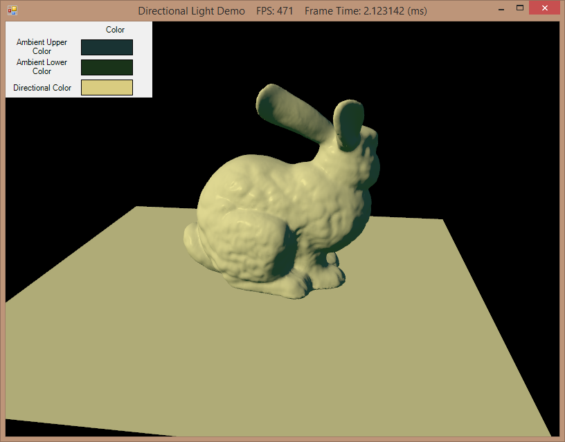
Below you can see a model being lit by directional light, in addition to the ambient lighting we used in the last example. Here, the directional light is coming downward and and from the lower-left to the upper-right. Surfaces with normals facing more directly towards the light source are lit more brightly than surfaces which are angled partly away from the light, while surfaces facing away from the light are lit only by ambient lighting. In addition, you can see a series of brighter spots along the back of the rabbit model, where there are specular highlights.
Full code for this example can be downloaded from my GitHub repository.
A Correction From the Previous Post
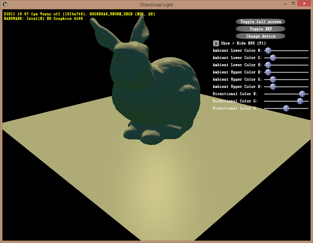
When I was working on converting the C++ sample code for the previous hemispherical ambient lighting example, I had a bunch of trouble getting the colors output by my code to match the original. I ended up getting this to work in that case by removing the step that converted the two ambient color values from gamma color-space to linear-space before passing them to the shader. However, when moving on to this directional lighting example, this no longer worked - summing the ambient light color with the directional light color in my pixel shader ended up doing some weird things, like the example below, where the lit surfaces appear blue-shifted.
 |
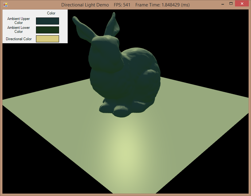 |
| Original C++ code output | My code without gamma correction |
After digging around and doing more shader debugging than I cared to, and researching gamma-correction (this and this were particularly helpful), I finally realized that the original C++ examples were using a different back-buffer format - R8G8B8A8_UNorm_SRGB vs the R8G8B8A8_UNorm I had been using. It's a little complicated, but if I understand what I have read (the two articles above, as well as this documentation on the the DXGI_FORMAT flags), essentially the plain UNORM format I had been using outputs colors in an unaltered gamma color-space, whereas the SRGB variant assumes colors are in linear color-space, and automatically performs a gamma-correction before rendering.
Once that was understood, it was relatively simple to get things working correctly. I made some changes to my application framework class, so that it is possible to use an SRGB backbuffer, by setting a flag in the constructor for each demo application that needs one, like so
GammaCorrectedBackBuffer = true;
I also needed to add in the function from the original examples which performs a gamma-to-linear color space conversion on color values that are passed to the shader.
private static Vector3 GammaToLinear(Vector3 c) {
    return new Vector3(c.X * c.X, c.Y * c.Y, c.Z * c.Z);
}
Strictly speaking, this is not totally correct, as the exponent used here ought to be 2.2, rather than 2, to match the gamma profile of most Windows displays, but simply squaring the color components is a little faster, and matches what is used in the original code.
Directional Lighting Effect
Our directional lighting effect is an evolution of the ambient lighting effect we used in the previous example. We have a new constant buffer to contain values (world-space camera eye location, material specular exponent and material specular intensity) specific to the directional lighting calculations that we will perform in our pixel shader, as well two additional lighting values for the directional light color and direction. We also have added a value for the world-space position of a vertex to our vertex shader output/pixel shader input structure.
cbuffer cbPerObject {
    float4x4 WorldViewProjection;
    float4x4 World;
    float4x4 gWorldInvTranspose;
};
// new
cbuffer cbPerObjectPS {
    float3 EyePosition;
    float specExp;
    float specIntensity;
};
cbuffer cbDirLightPS {
    float3 AmbientDown;
    float3 AmbientRange;
    float3 DirToLight; // new
    float3 DirLightColor; // new
};
Texture2D DiffuseTexture;
SamplerState LinearSampler {
    Filter = MIN_MAG_MIP_LINEAR;
    AddressU = WRAP;
    AddressV = WRAP;
    AddressW = WRAP;
    MaxAnisotropy = 1;
};
struct VS_INPUT {
    float3 Position : POSITION;
    float3 Normal : NORMAL;
    float2 UV : TEXCOORD0;
};
struct VS_OUTPUT {
    float4 Position : SV_POSITION;
    float2 UV : TEXCOORD0;
    float3 Normal : TEXCOORD1;
    float3 WorldPos : TEXCOORD2; // new
};
Our vertex shader will be modified to calculate the world-space position of each vertex and store this in the new VS_OUTPUT.WorldPos field. This is a simple object-to-world transformation.
VS_OUTPUT RenderSceneVS(VS_INPUT input) {
    VS_OUTPUT output;
    float3 vNormalWorldSpace;
    output.Position = mul(float4(input.Position, 1.0f), WorldViewProjection);
    // new
    output.WorldPos = mul(float4(input.Position, 1.0f), World).xyz;
    output.UV = input.UV;
    output.Normal = mul(input.Normal, (float3x3)gWorldInvTranspose);
    return output;
}
We'll also introduce a material structure to encapsulate the surface properties of the mesh being rendered. This is somewhat less simpler but less flexible than the material structure I have used in my earlier Luna-based examples, but follows the same general idea. This structure contains fields for the surface normal, diffuse color, specular exponent and specular intensity. We will also create a helper function to manufacture an instance of this structure, based upon the normal and texture UV coordinates of our VS_OUTPUT structure, which will be used by our pixel shader.
struct Material {
    float3 normal;
    float4 diffuseColor;
    float specExp;
    float specIntensity;
};
Material PrepareMaterial(float3 normal, float2 UV) {
    Material material;
    material.normal = normalize(normal);
    material.diffuseColor = DiffuseTexture.Sample(LinearSampler, UV);
    // gamma correct input texture diffuse color to linear-space
    material.diffuseColor.rgb *= material.diffuseColor.rgb;
    material.specExp = specExp;
    material.specIntensity = specIntensity;
    return material;
}
Next, we have our directional light pixel shader. This makes use of the PrepareMaterial() function above to prepare the surface properties structure, then calculates the ambient lighting, in the same manner as in our previous example, and then calculates the directional lighting using the CalcDirectional() helper function.
float3 CalcDirectional(float3 position, Material material) {
    // calculate diffuse light
    float NDotL = dot(DirToLight, material.normal);
    float3 finalColor = DirLightColor.rgb * saturate(NDotL);
    // calculate specular light and add to diffuse
    float3 toEye = EyePosition.xyz - position;
    toEye = normalize(toEye);
    float3 halfway = normalize(toEye + DirToLight);
    float NDotH = saturate(dot(halfway, material.normal));
    finalColor += DirLightColor.rgb * pow(NDotH, material.specExp) * material.specIntensity;
    // scale light color by material color
    return finalColor * material.diffuseColor.rgb;
}
float4 DirectionalLightPS(VS_OUTPUT input) :SV_TARGET0{
    Material material = PrepareMaterial(input.Normal, input.UV);
    float3 finalColor = CalcAmbient(material.normal, material.diffuseColor.rgb);
    finalColor += CalcDirectional(input.WorldPos, material);

    return float4(finalColor, 1.0);
}
Our CalcDirectional() function calculates the direct lighting using the Blinn-Phong reflection model. This reflectance model uses the vectors shown below to calculate the diffuse and specular lighting components.

- N - The surface normal vector.
- L - The vector from the surface to the light source.
- V - The vector from the surface to the camera location.
- R - The direction that specular highlights will be reflected.
- H - The vector half-way between the view and light vectors.
Calculating the diffuse component of the directional light is pretty straightforward. Conceptually, what we are doing here is calculating how directly the light source is shining on the surface. If you recall your linear algebra, the dot product of two normalized vectors is equal to the cosine of the angle between them. This makes the dot product perfect for determining how directly the light is shining on the surface, as a few cases should illustrate:
- Normal and To-Light are the same - dot(N, L) = 1, so the surface should be fully lit by the light.
- Normal and To-Light are in the same plane - 0 < dot(N, L) < 1, so the surface is partially lit.
- Normal and To-Light are perpendicular - dot(N, L) = 0, so the surface is not lit.
- Normal and To-Light face away from each other - dot(N, L) < 0, so the surface is not lit.
Calculating the specular lighting is more complex. The classic Phong reflection model uses only the L, N, V and R vectors in the above diagram. Because calculating the reflected vector R can be computationally expensive, the Blinn-Phong model uses a heuristic to simplify the calculation. Rather than calculate the reflection vector directly, we calculate the vector that lies halfway between the view (V) and light (L), which is H in the diagram above. Physically, we can understand the halfway vector H as the normal of a surface that would reflect light cast from the light source directly to the camera's position. Thus, we can use dot(N, H) as a measure of how close the actual surface normal is to the ideally reflecting normal described by H, and thus the base intensity factor of the reflected light, similar to how we calculated the diffuse lighting.
Once we have calculated dot(N, H), we raise it to the power specified by the specular exponent shader constant, scale it by the specular intensity shader constant, and use the resulting value to scale the light intensity of the directional light, to obtain the final specular light component, which we add to the diffuse lighting component. The specular exponent in this equation controls the size of the specular highlights - smaller specular exponents result in larger, softer highlights, whereas larger exponents will result in smaller, tighter highlights.
The last thing we must do in our shader code is define an effect technique to use our new directional lighting pixel shader.
technique11 Directional {
    pass P0 {
        SetVertexShader(CompileShader(vs_5_0, RenderSceneVS()));
        SetPixelShader(CompileShader(ps_5_0, DirectionalLightPS()));
    }
}
Since this is already getting rather lengthy, and there is very little that is very interesting about the demo application code outside of the shaders, I'm going to skip ahead and just leave you with a video showing the output. Notice how the specular highlights shift as the camera moves around the scene. You can play around with different light directions, specular exponents and specular intensities in the code to get a better idea of how these values modify the computed lighting.
Next Time...
Next up, we'll move on to examining point light sources.